Fibonacci Numbers Case Study

Everyone rolls their eyes at Fibonacci numbers because they’re the cliché interview question nobody uses on a trading desk. But as an autopsy on Python execution speed, nothing exposes the hidden costs of call-stack frames, object allocation, and algorithmic complexity quite like it.

Let’s take the textbook recursive definition, watch it bring our CPU to its knees for trivial inputs, and systematically re-engineer it until it runs at hardware limits.

Naive Recursive Approach

The Fibonacci sequence is defined by the recurrence relation: \(F_n = F_{n-1} + F_{n-2}\) with seed values \(F_0=0\) and \(F_1=1\).

A naive implementation of this in Python is a direct translation of the mathematical formula:

Show the code

def fibonacci_recursive(n: int) -> int:
    """Calculate the nth Fibonacci number using a recursive approach."""
    if n < 0:
        raise ValueError("Fibonacci is not defined for negative numbers.")
    if n < 2:
        return n
    return fibonacci_recursive(n - 1) + fibonacci_recursive(n - 2)

This approach is very intuitive, but it is also very slow. For n=40, it already takes a noticeable amount of time to compute. The reason is that the function calls itself twice for each n, leading to an exponential explosion of stack frames (\(O(2^n)\)).

Show the code

from time import perf_counter

start = perf_counter()
_ = fibonacci_recursive(40)
end = perf_counter()

print(f"Execution took {end - start:.2f} seconds")

Execution took 20.78 seconds

Visualizing the Call Stack

To better understand the problem, let’s visualize the call stack. We can create a “talkative” version of our function that logs every call.

Show the code

from rich.console import Console
from rich.tree import Tree


def fibonacci_recursive_talkative(n: int) -> int:
    """Calculate the nth Fibonacci number using a recursive approach."""
    tree = Tree(f"fibonacci_recursive_talkative({n})")

    def worker(n: int, tree: Tree) -> int:
        """Calculate the nth Fibonacci number using a recursive approach."""
        node = tree.add(f"fibonacci_recursive({n}) called")
        if n < 0:
            raise ValueError("Fibonacci is not defined for negative numbers.")
        if n < 2:
            return n
        return worker(n - 1, node) + worker(n - 2, node)

    result = worker(n, tree)
    Console().print(tree)
    return result

For n=6, the call tree looks like this:

Show the code

_ = fibonacci_recursive_talkative(6)

fibonacci_recursive_talkative(6)
└── fibonacci_recursive(6) called
    ├── fibonacci_recursive(5) called
    │   ├── fibonacci_recursive(4) called
    │   │   ├── fibonacci_recursive(3) called
    │   │   │   ├── fibonacci_recursive(2) called
    │   │   │   │   ├── fibonacci_recursive(1) called
    │   │   │   │   └── fibonacci_recursive(0) called
    │   │   │   └── fibonacci_recursive(1) called
    │   │   └── fibonacci_recursive(2) called
    │   │       ├── fibonacci_recursive(1) called
    │   │       └── fibonacci_recursive(0) called
    │   └── fibonacci_recursive(3) called
    │       ├── fibonacci_recursive(2) called
    │       │   ├── fibonacci_recursive(1) called
    │       │   └── fibonacci_recursive(0) called
    │       └── fibonacci_recursive(1) called
    └── fibonacci_recursive(4) called
        ├── fibonacci_recursive(3) called
        │   ├── fibonacci_recursive(2) called
        │   │   ├── fibonacci_recursive(1) called
        │   │   └── fibonacci_recursive(0) called
        │   └── fibonacci_recursive(1) called
        └── fibonacci_recursive(2) called
            ├── fibonacci_recursive(1) called
            └── fibonacci_recursive(0) called

Look at that tree. To compute \(F(6)\), our code evaluates \(F(4)\) twice and \(F(3)\) three times. By the time you ask for \(F(40)\), Python evaluates over 300 million identical subtrees from scratch.

What if our function had a memory? Before computing anything, what if it glanced at a simple lookup table to see if it already solved that exact subproblem?

Memoization

Storing intermediate results in a dictionary cache transforms this exponential nightmare into linear execution (\(O(n)\)). This technique is called memoization:

Show the code

FIBONACCI_CACHE: dict[int, int] = {}


def fibonacci_recursive_cached(n: int) -> int:
    """Calculate the nth Fibonacci number using recursion with memoization."""
    if n < 0:
        raise ValueError("Fibonacci is not defined for negative numbers.")
    if n < 2:
        return n

    if n in FIBONACCI_CACHE:
        return FIBONACCI_CACHE[n]

    result = fibonacci_recursive_cached(n - 1) + fibonacci_recursive_cached(n - 2)

    FIBONACCI_CACHE[n] = result
    return result

This version is much faster. However, it will fail for large n (e.g., n=8_000) because of Python’s recursion depth limit.

Show the code

try:
    fibonacci_recursive_cached(8_000)
except RecursionError as e:
    print(e)

maximum recursion depth exceeded

Decorators for Caching

A more elegant way to implement memoization is by using a decorator. A decorator is a function that takes another function and extends its behavior without explicitly modifying it. Python’s functools module provides a built-in decorator lru_cache that does exactly what we need.

Show the code

from functools import cache


@cache
def fibonacci_recursive_cached_decorator(n: int) -> int:
    """Calculate the nth Fibonacci number using recursion with memoization."""
    if n < 0:
        raise ValueError("Fibonacci is not defined for negative numbers.")
    if n < 2:
        return n
    return fibonacci_recursive_cached_decorator(
        n - 1
    ) + fibonacci_recursive_cached_decorator(n - 2)

This is the most concise and Pythonic way to write a cached recursive Fibonacci function.

Iterative Approach

Another way to solve the problem is to use an iterative approach. This is equivalent to tail recursion optimization.

Show the code

def fibonacci_iterative(n: int) -> int:
    """Calculate the nth Fibonacci number using an iterative approach."""
    if n < 0:
        raise ValueError("Fibonacci is not defined for negative numbers.")
    if n < 2:
        return n

    a, b = 0, 1
    for _ in range(n - 1):
        a, b = b, a + b
    return b

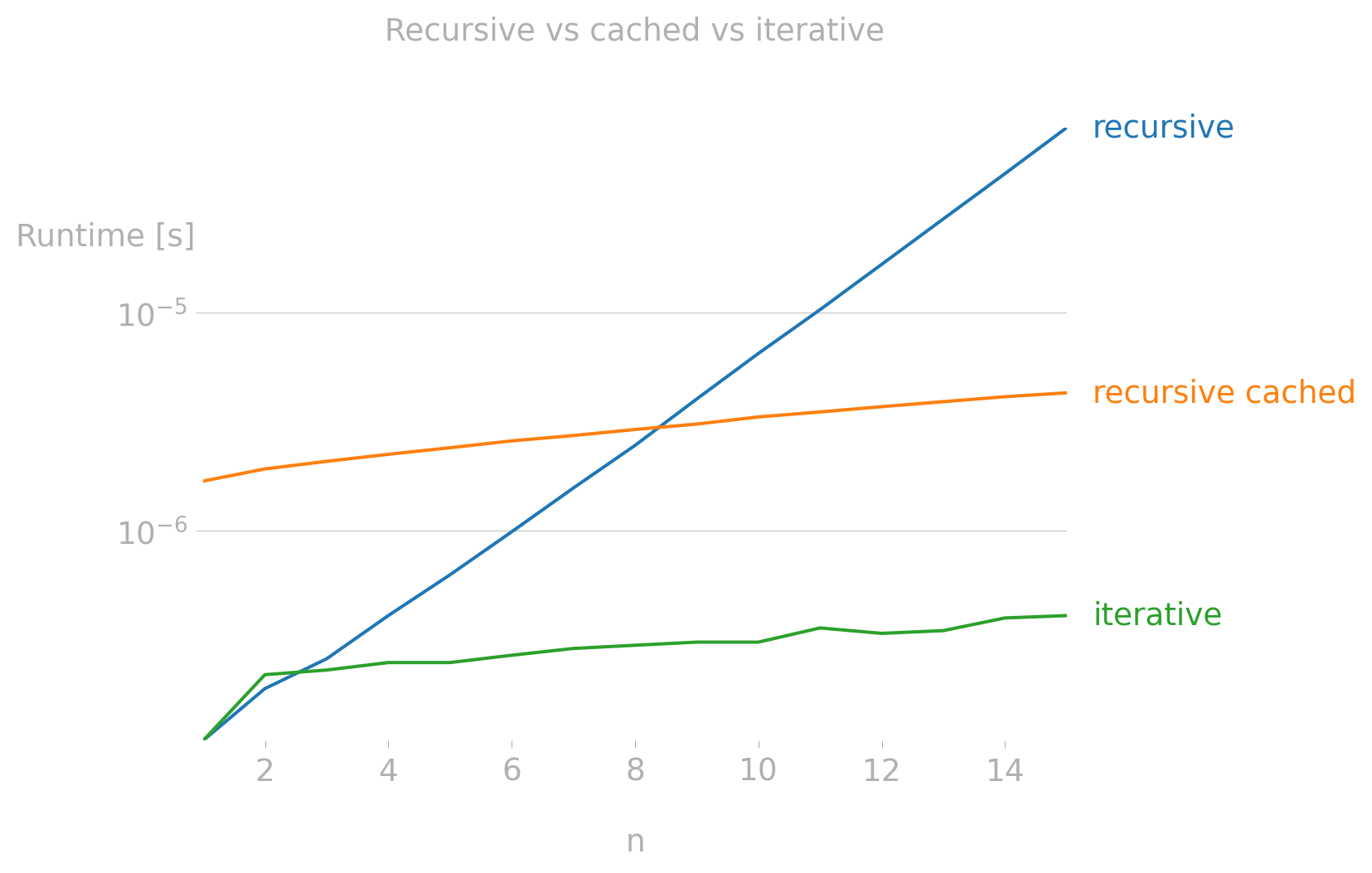
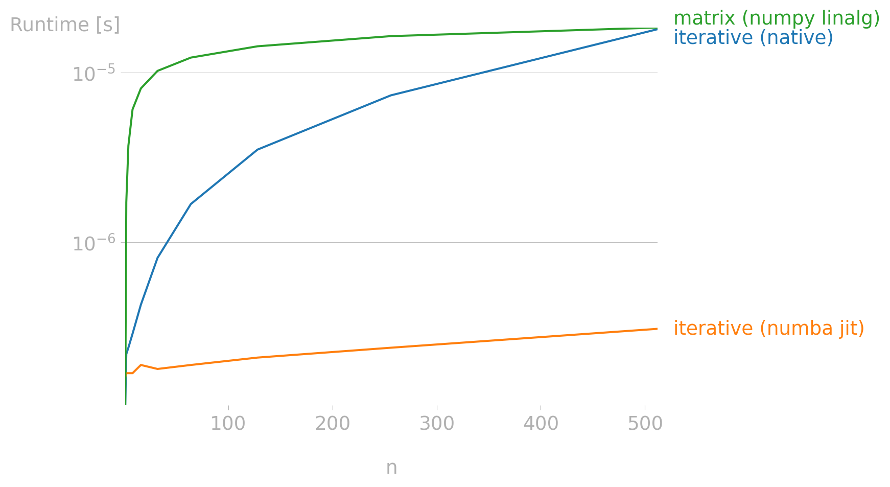
This is a clean, linear-time \(O(n)\) solution with constant \(O(1)\) space. As we will see in the benchmarks, while matrix exponentiation can reduce time complexity to \(O(\log n)\), a tight iterative loop in Python or Numba is hard to beat for practical integer sizes.

Performance Comparison

To compare the performance of these implementations, we can use the perfplot library. It allows us to easily benchmark different functions over a range of input sizes.

Show the code

import numba
import perfplot
import numpy as np


def fibonacci_internal_cached_decorator(n: int) -> int:
    """Calculate the nth Fibonacci number using recursion with memoization.

    This version uses an internal helper function decorated with @cache.
    This forces the cache to be local to this function.
    """

    @cache
    def helper(n: int) -> int:
        """Calculate the nth Fibonacci number using recursion with memoization."""
        if n < 0:
            raise ValueError("Fibonacci is not defined for negative numbers.")
        if n < 2:
            return n
        return helper(n - 1) + helper(n - 2)

    return helper(n)


fibonacci_iterative_jit = numba.njit(fibonacci_iterative)

1_ = fibonacci_iterative_jit(10)


def fibonacci_linalg_numpy(n):
    """Calculate the nth Fibonacci number using matrix exponentiation with NumPy."""

    if n <= 0:
        return 0
    if n == 1:
        return 1

    Q = np.array([[1, 1], [1, 0]], dtype=np.uint64)
2    result_matrix = np.linalg.matrix_power(Q, n - 1)
    return result_matrix[0, 0]

1: Warm-up call to trigger JIT compilation before benchmarking.
2: Binary matrix exponentiation reduces theoretical time complexity to \(O(\log n)\).

Show the code

perfplot.show(
    setup=lambda n: n,
    kernels=[
        fibonacci_recursive,
        fibonacci_internal_cached_decorator,
        fibonacci_iterative,
    ],
    n_range=[i for i in range(1, 16)],
    xlabel="n",
    labels=[
        "recursive",
        "recursive cached",
        "iterative",
    ],
    title="Recursive vs cached vs iterative",
    show_progress=False,
    equality_check=False,
    logx=False,
    logy=True,
)

There are more advanced techniques and algorithms to compute Fibonacci numbers, below is a sneak peek for the future at two more efficient methods: using Numba’s JIT compilation and matrix exponentiation with NumPy.

Show the code

perfplot.show(
    setup=lambda n: n,
    kernels=[
        fibonacci_iterative,
        fibonacci_iterative_jit,
        fibonacci_linalg_numpy,
    ],
    n_range=[2**i for i in range(10)],
    xlabel="n",
    labels=[
        "iterative (native)",
        "iterative (numba jit)",
        "matrix (numpy linalg)",
    ],
    equality_check=False,
    show_progress=False,
    logx=False,
    logy=True,
)

In the next post, we’ll use these Fibonacci implementations to explore first-class functions, closures, and decorators.

Note

Download the whole code here.